mrvplot Package Demo

library(mrvplot)
library(ggplot2)
library(dplyr)
#> 
#> Attaching package: 'dplyr'
#> The following objects are masked from 'package:stats':
#> 
#>     filter, lag
#> The following objects are masked from 'package:base':
#> 
#>     intersect, setdiff, setequal, union

This vignette demonstrates the plotting functions available in the mrvplot package.

Theme Functions

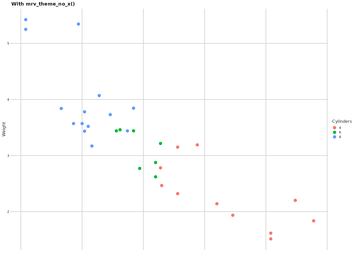
The package provides several theme wrappers with consistent font sizing:

# Sample data
p <- ggplot(mtcars, aes(mpg, wt)) +
  geom_point(aes(color = factor(cyl))) +
  labs(
    title = "Miles per Gallon vs Weight",
    x = "MPG", y = "Weight", color = "Cylinders"
  )

# Different grid themes
p + mrv_grid() + ggtitle("mrv_grid()")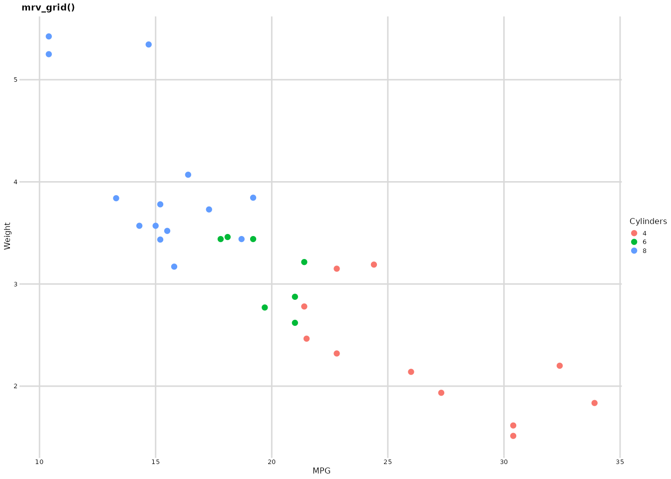

p + mrv_hgrid() + ggtitle("mrv_hgrid()")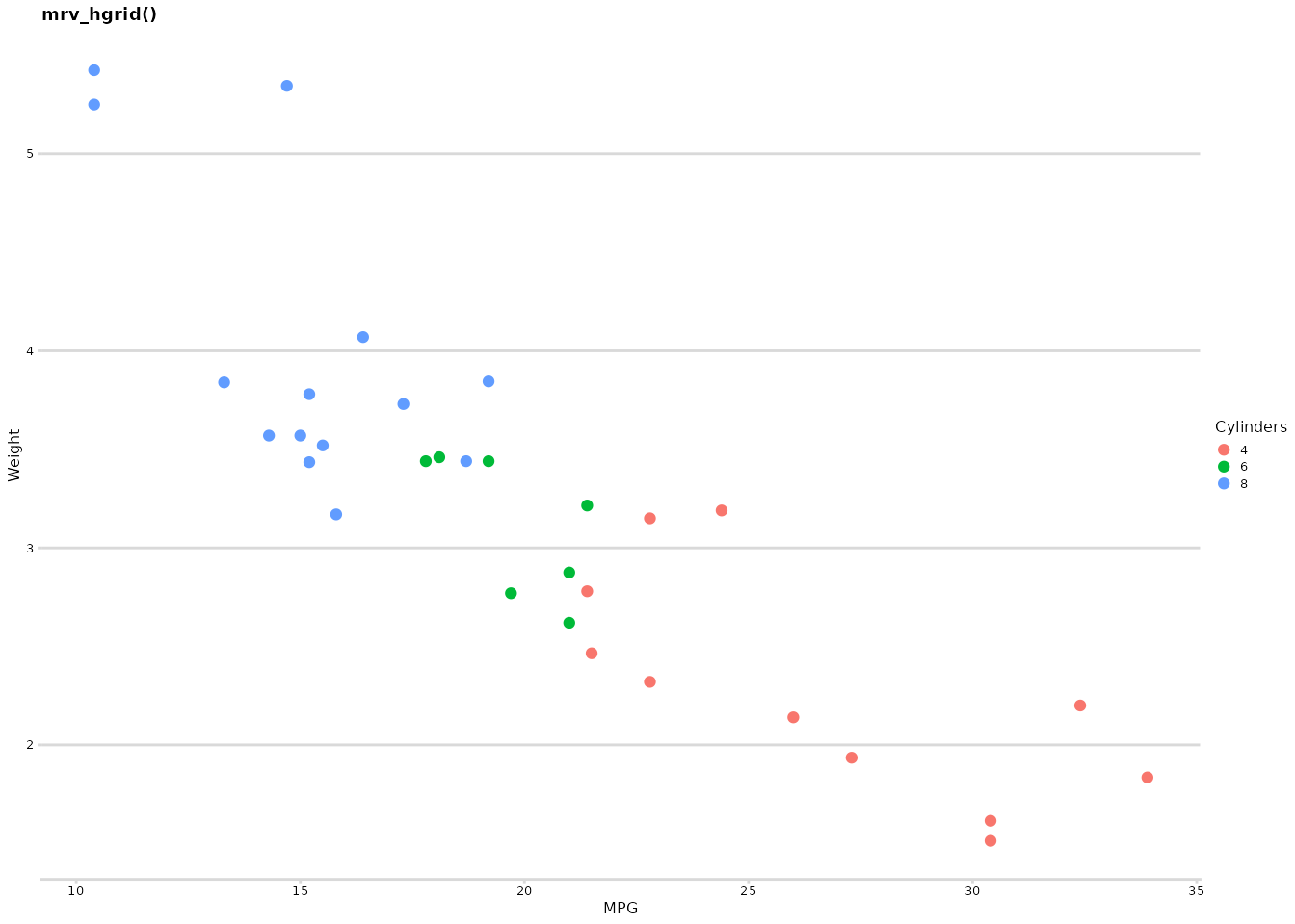

p + mrv_vgrid() + ggtitle("mrv_vgrid()")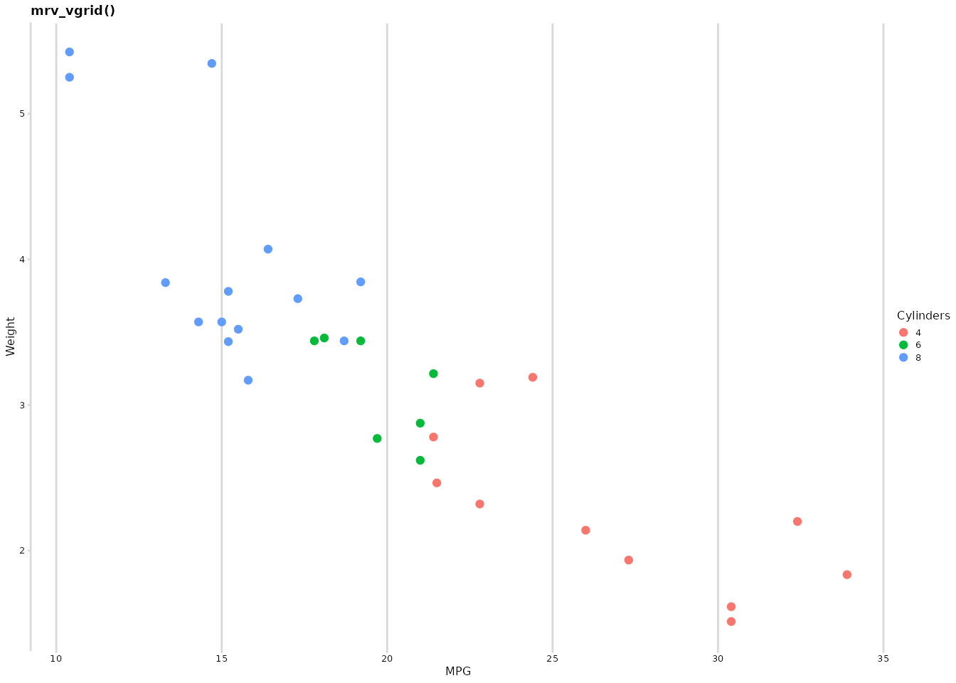

Removing X-Axis Elements

p + mrv_grid() + mrv_theme_no_x() + ggtitle("With mrv_theme_no_x()")

Enhanced ggsave

The mrv_ggsave() function saves plots while also exporting data:

# This will save the plot and create a Tables/ directory with data
p + mrv_grid()
mrv_ggsave("Figures/demo_plot.pdf", width = 3, height = 2)

Transformation Functions

Reverse Log Transform

# Create data with exponential relationship
df <- data.frame(x = 1:100, y = exp(-(1:100) / 20))

ggplot(df, aes(x, y)) +
  geom_line() +
  scale_y_continuous(trans = reverselog_trans()) +
  mrv_grid() +
  labs(title = "Reverse Log Transform", y = "Reverse Log Scale")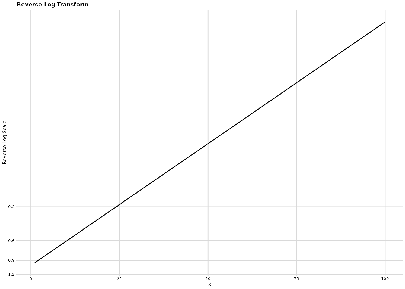

Scientific Notation

# Data with large numbers
large_data <- data.frame(
  x = c(1e3, 1e6, 1e9, 1e12),
  y = c(2, 4, 6, 8)
)

ggplot(large_data, aes(x, y)) +
  geom_point(size = 3) +
  scale_x_log10(labels = scientific_10) +
  mrv_grid() +
  labs(title = "Scientific Notation Labels", x = "Value (log scale)")

Utility Functions

Reading BED Files

# Example of reading a BED file (file not included in demo)
# bed_data <- mrv_read_bed("sample.bed")
# head(bed_data)